By: Syed Islam
Introduction
Data transformation and cleansing are important parts of data engineering and analytics. They involve changing raw data into a more useful format for analysis. In this blog post, we’ll look at some practical examples of data cleansing and transformation using PySpark within Microsoft Fabric’s Notebook environment.
Microsoft Fabric
Microsoft Fabric is an end-to-end analytics and data platform that integrates various data services (such as Power BI, Azure Synapse Analytics, and Azure Data Factory) into a single, unified environment. This integration simplifies data management, analytics, and governance, providing a seamless experience for data professionals.
PySpark
PySpark is the Python API for Apache Spark, a powerful system for processing and analyzing large amounts of data. PySpark allows users to leverage Spark’s advanced data processing capabilities, making it easier for more data scientists and engineers to use.
Fabric Notebooks
Notebooks in Microsoft Fabric provide an interactive environment for data exploration, analysis, and visualization. They support multiple languages (including Python) and integrate seamlessly with other Microsoft Fabric services, which makes them an ideal tool for data professionals.
Step-by-Step Guide to Data Cleansing and Transformation
Step 1: Log in to the Microsoft Fabric Portal
Log in to your Microsoft Fabric account (if you don’t have one, you can sign up for a trial to explore its features). Select “Synapse Data Engineering” experience. 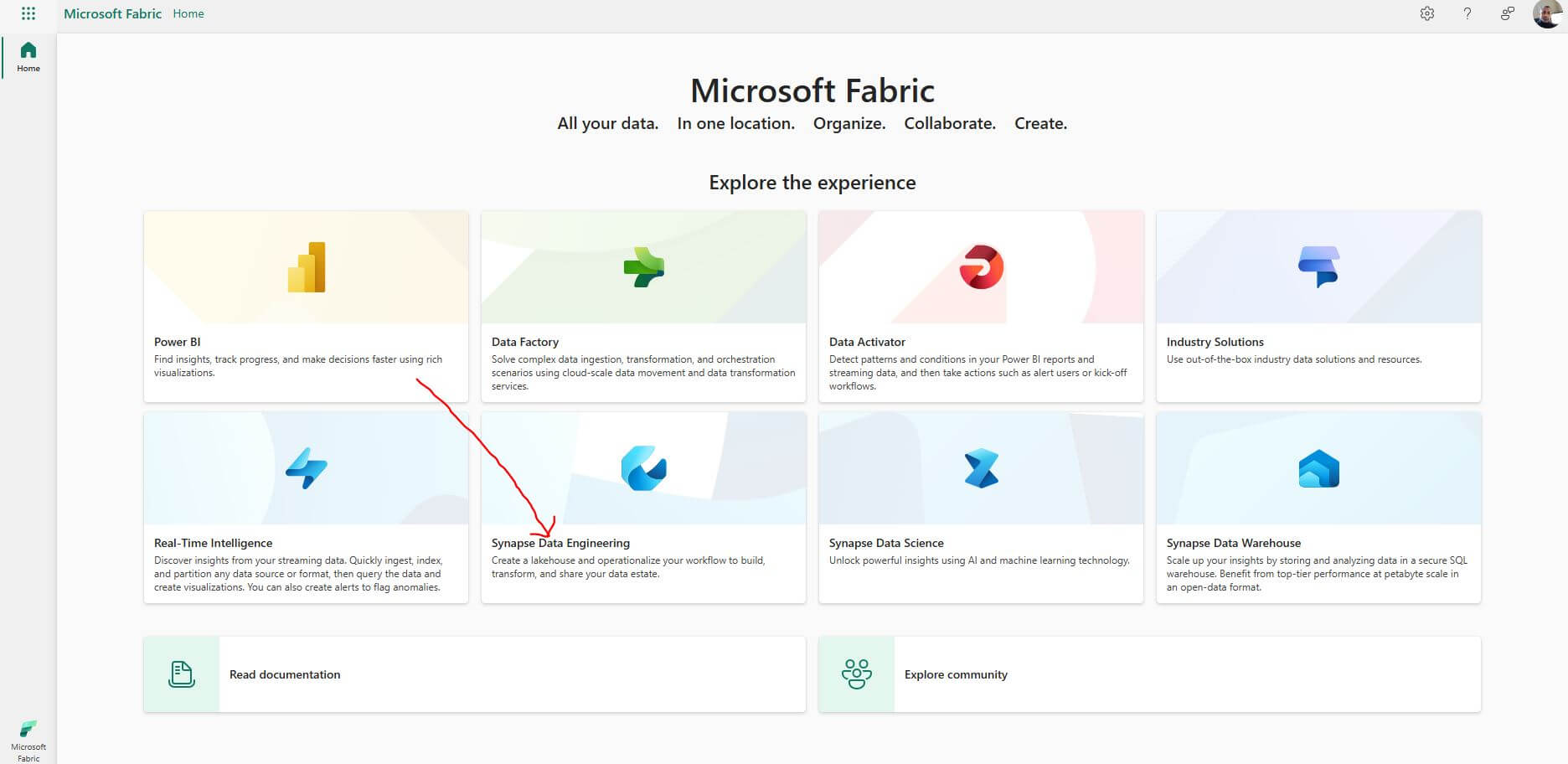
Step 2: Creating a New Notebook in Microsoft Fabric
Select “New item” from the top menu. Select “Notebook” button from the list of available items. 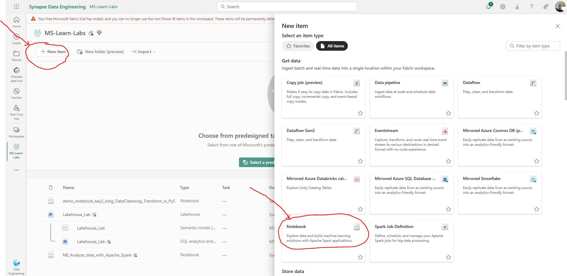 This will create a brand new notebook. Let’s rename the notebook with a more meaningful title.
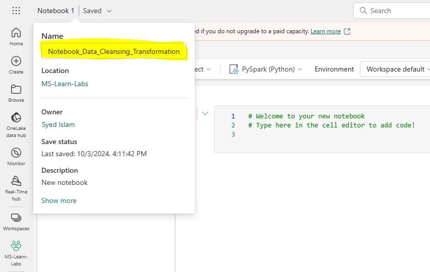
Step 3: Loading Data
Select “Upload files” from the Lakehouse explorer “File” section. 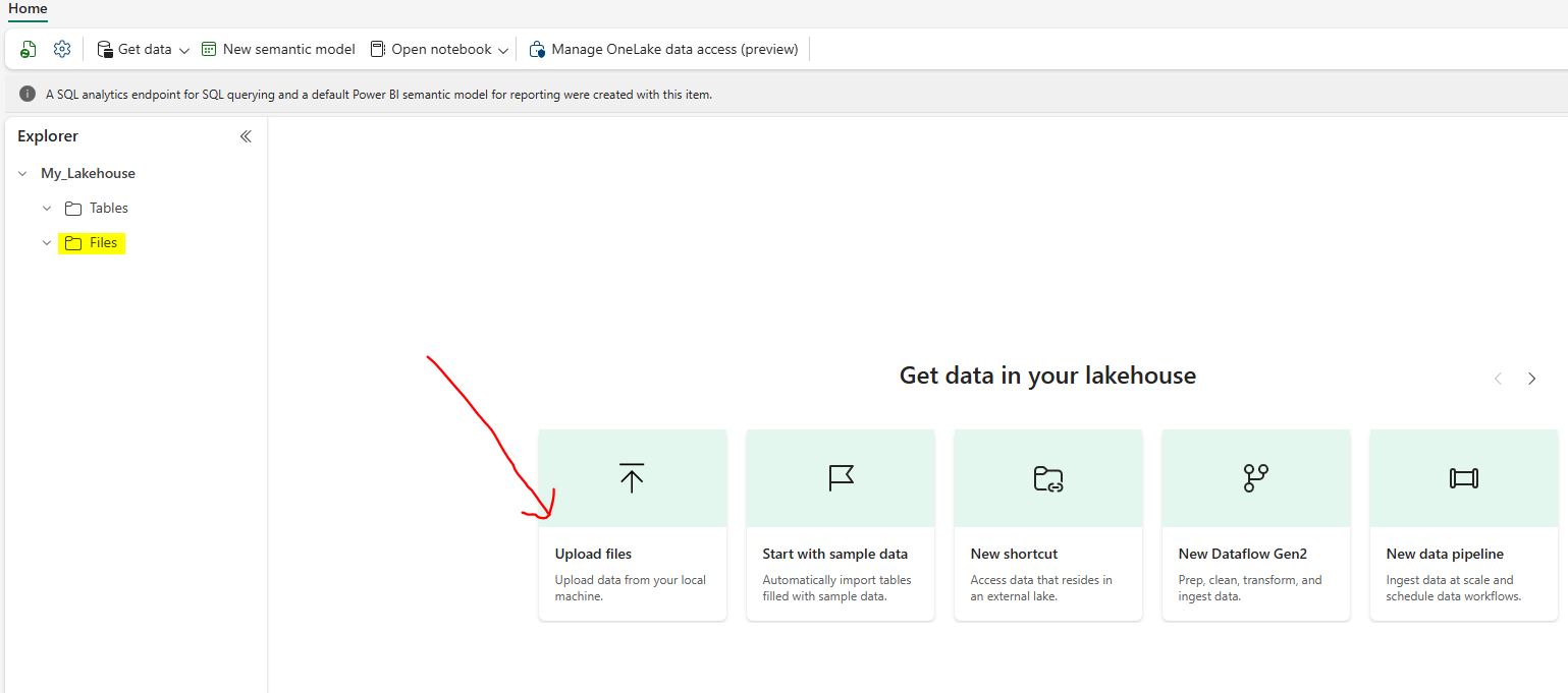 From the “Upload files” dialog window, select sample data files “Customers.csv” & “Orders.csv”.
 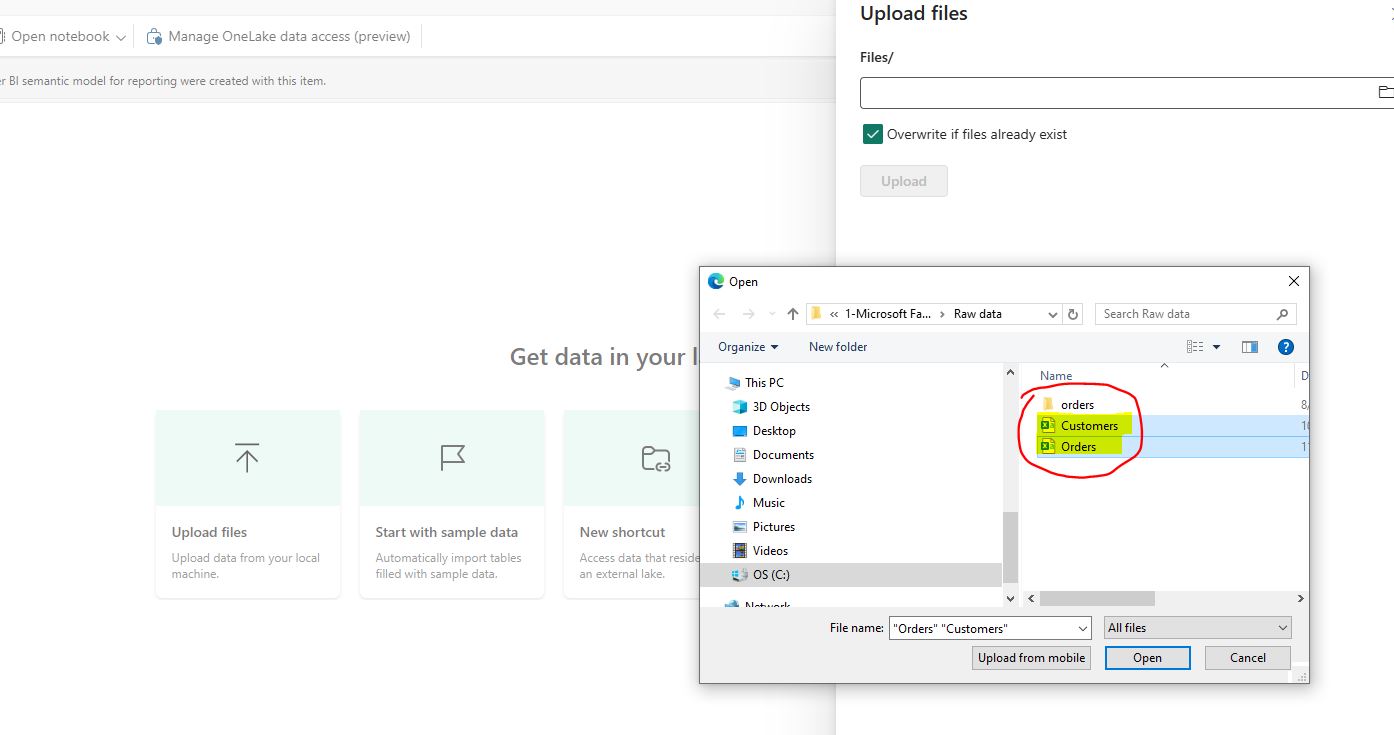 Select checkbox: “Overwrite if files already exist.” Select the “Upload” button.
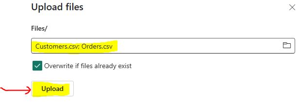
Step 4: Exploring Datasets
Let’s explore the two datasets we just loaded into the Fabric Lakehouse. 4.1 Displaying the Datasets: Shows samples of the Orders and Customers datasets to understand their structure and content. Open the notebook we created in Step 2. Write or copy the following PySpark code into the notebook to display the “Orders” dataset: df_orders = spark.read.format(“csv”).option(“header”,”true”).load(“Files/Orders.csv”) display(df_orders) Click Run cell play button. It should return the following table: 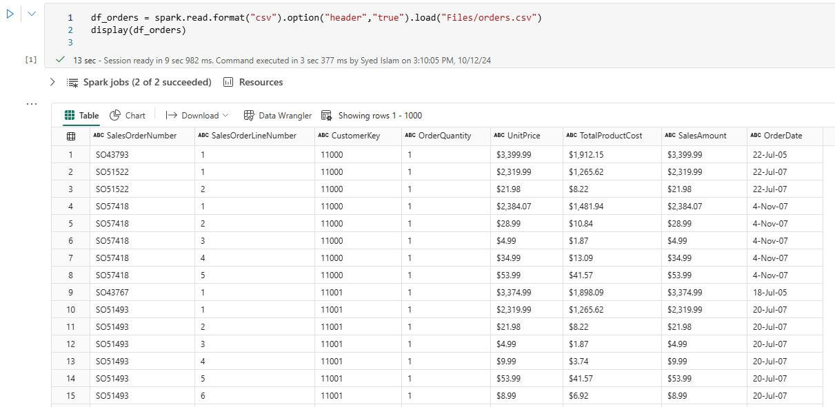 Next, write or copy the following PySpark code into the notebook to display the ‘Customer’ dataset: df_cust = spark.read.format(“csv”).option(“header”,”true”).load(“Files/Customers.csv”) display(df_cust) Click Run cell play button. It should return the following table:
 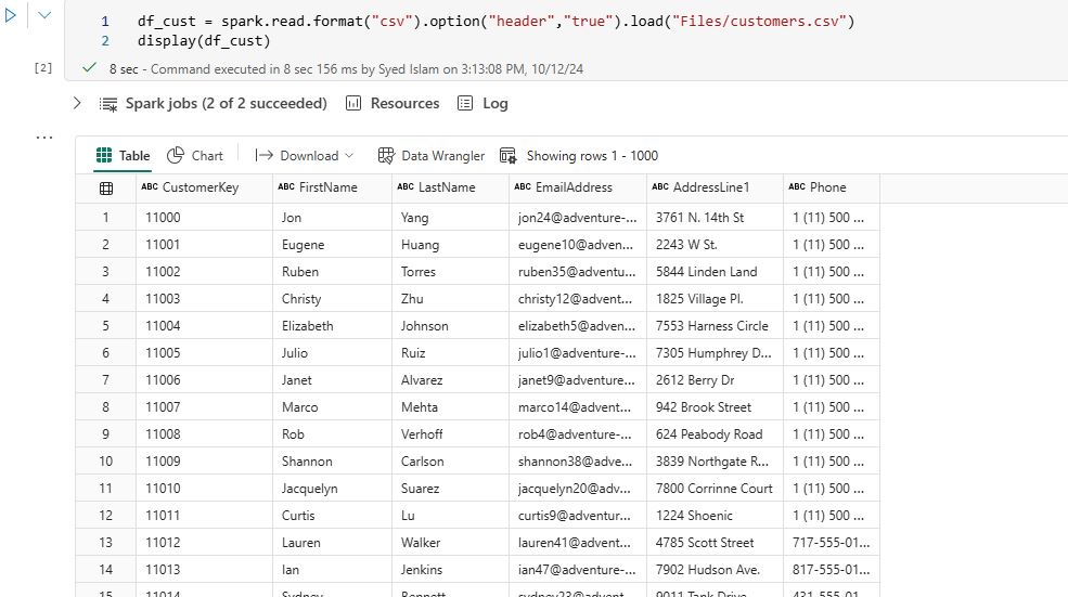 4.2 Counting rows: Determining the total number of rows in the datasets to assess their size. Write or copy the following PySpark code into the notebook to display total row counts for ‘Orders’ and ‘Customers’ datasets: df_orders.count() df_cust.count()
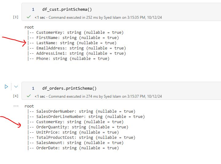
  4.3 Schema Information: Displaying the schema to reveal the data types and structure of the dataset. Write or copy the following code into the notebook to show schemas for ‘Orders’ and ‘Customers’ tables: df_cust.printSchema() df_orders.printSchema() Click Run cell play button. It should return the following table schema info:
Step 5: Data Cleansing
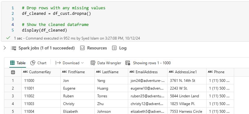
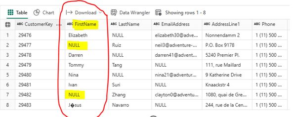
4.1 Handling Missing Values: Identify and handle missing values in your dataset. You can choose to drop rows with missing values or fill them with appropriate values: # Drop rows with any missing values The following rows from the Customer table contain null values that need to be removed: 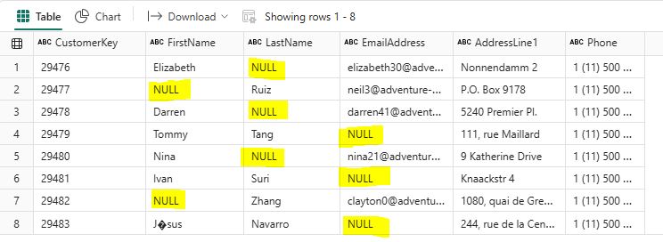 Write the following PySpark code to remove rows that contain missing values. The cleaned DataFrame is displayed, showing only rows without missing values: # Drop rows with any missing values df_cleaned = df_cust_new_rows.dropna() # Show the cleaned dataframe: display(df_cleaned)
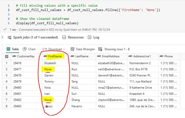
  # Fill missing values with a specific value In PySpark, you can use the fillna method to replace null or missing values in a specific column. For the FirstName column, you can fill missing values with the string “None”. Write the following PySpark code to fill missing values in the FirstName column df_cust = df.fillna({‘FirstName’: ‘None’})
  After running the scripts, null values are replaced with ‘None’:
  4.2 Removing Duplicates: Ensure your data is free from duplicates to maintain data integrity. Duplicates can affect results and cause inefficiencies. The following rows in the Customer data frame contain duplicates that need to be removed:
 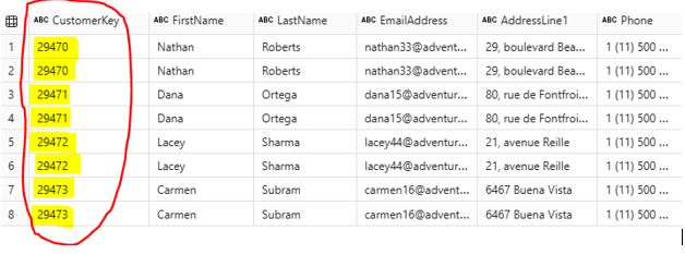 Write the following PySpark scripts to remove duplicates: # Drop duplicates df_drop_duplicate = df_cust.dropDuplicates() After running the scripts, the duplicates have been removed:
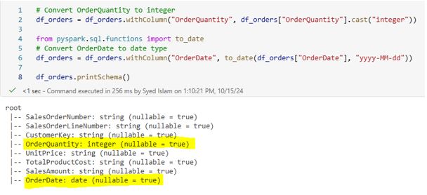
  4.3 Correcting Data Types: Making sure that each column in your DataFrame has the correct data type is crucial for accurate data analysis and processing. Incorrect data types can lead to errors in calculations, misinterpretation of data, and inefficient processing. PySpark provides powerful tools to inspect and correct data types in your DataFrame. Write the following PySpark scripts to convert two of the data types. df_orders = df_orders.withColumn(“OrderQuantity”, df_orders[“OrderQuantity”].cast(“integer”)) from pyspark.sql.functions import to_date df_orders = df_orders.withColumn(“OrderDate”, to_date(df_orders[“OrderDate”], “yyyy-MM-dd”))
Step 6: Data Transformation
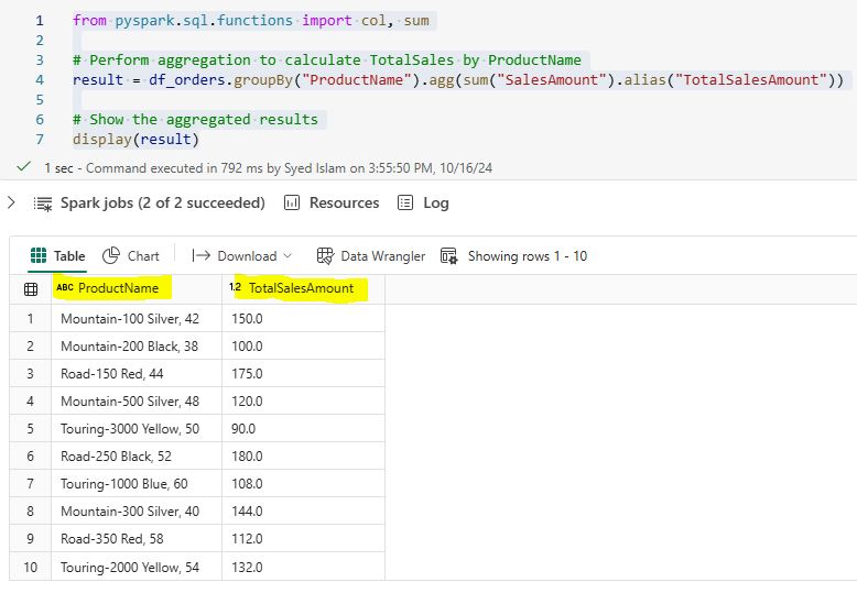
5.1 Feature Engineering: Create new features that can provide additional insights in your dataset. For example, we can create a new column FullName by concatenating the FirstName and LastName columns. Write the following PySpark scripts to add a new column. from pyspark.sql.functions import col, concat_ws df_cust_fullname = df_cust.withColumn(“FullName”, concat_ws(” “, col(“FirstName”), col(“LastName”))) display(df_cust_fullname) 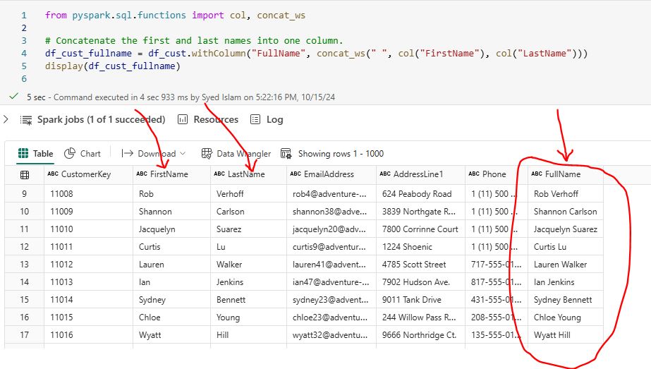 5.2 Data Aggregation: Aggregating data is a fundamental step in data analysis. It lets you summarize your data and find useful insights. PySpark provides powerful functions to perform various aggregation operations such as sum, average, count, min, and max. These functions help in transforming raw data into meaningful summaries. For example, you can calculate the total sales per product using PySpark: from pyspark.sql.functions import col, sum result = df_orders.groupBy(“ProductName”).agg(sum(“SalesAmount”).alias(“TotalSalesAmount”)) display(result)
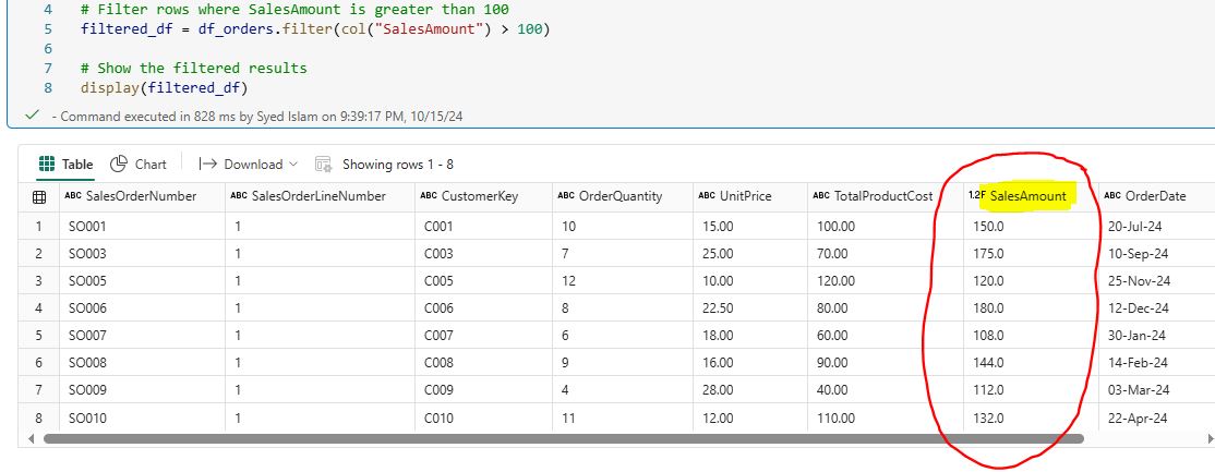
  5.3 Filtering Data: Filtering data is a crucial step in data analysis, allowing you to focus on specific subsets of your dataset that meet certain conditions. PySpark provides powerful functions to filter rows based on various criteria, making it easy to work with only the relevant data. For example, you can filter orders with a sales amount greater than 100 using PySpark: from pyspark.sql.functions import col filtered_df = df_orders.filter(col(“SalesAmount”) > 100) display(filtered_df)
  5.4 Joining DataFrames: Joining DataFrames allows you to enrich your dataset by adding columns from the second DataFrame that match rows in the first. For example, combining customer information with transaction details on
 customer_key provides a comprehensive view of each customer’s transactions: joined_df = df_cust.join(df_orders, df_cust[“CustomerKey”] == df_orders[“CustomerKey”], “inner”) result = df_joined.select( col(“FirstName”), col(“LastName”), col(“SalesOrderNumber”), col(“OrderQuantity”), col(“SalesAmount”), col(“OrderDate”) ) display(result) 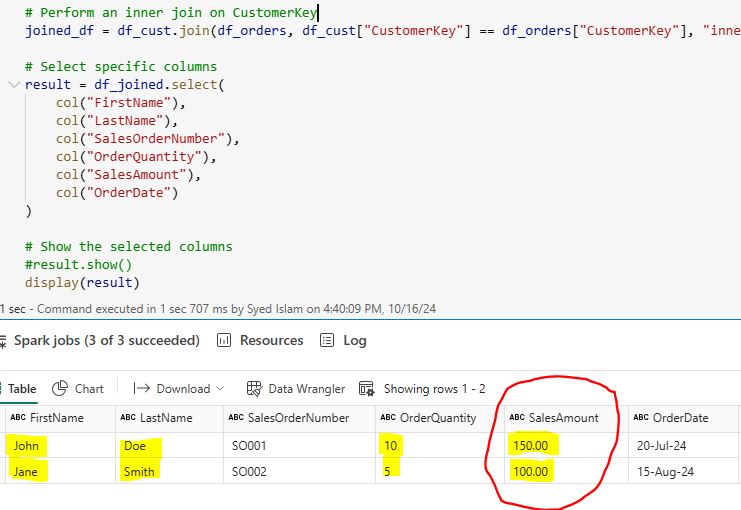
Conclusion
Performing data cleansing and transformation with PySpark in Microsoft Fabric allows you to leverage the strengths of both platforms. PySpark provides powerful data processing capabilities, while Microsoft Fabric offers a unified environment for data management, analytics, and visualization. By following these steps, you can build robust data pipelines that drive insights and support decision-making in your organization.

